Do you actually need a vector database?
Brute-force cosine similarity over vectors in SQLite stays under 100 ms to roughly 300,000 rows at 384 dimensions — if the dot product is not running in a Python loop, where the same wall arrives seventeen times earlier. Measured latency, storage and what an HNSW index actually buys.

Brute-force cosine similarity over every row stays inside a 100 ms budget up to about 300,000 vectors at 384 dimensions — but only if the dot product is not running in a Python loop, where the same wall arrives at roughly 18,000. The number that decides this is not your row count. It is how many bytes per second your scan can read.
Everything below uses randomly generated vectors. That is a real limitation and it needs saying before any number appears. Random vectors give perfectly valid performance numbers — a dot product costs the same regardless of what the floats mean — but they say nothing whatsoever about retrieval quality. No claim about relevance, recall on real data, or whether search results are any good is made anywhere in this article, and one measurement below shows exactly how badly random data misleads you if you try. There is no embedding API call here, no model, no network.
Hardware: Apple M3, 16 GB, macOS 26.4.1. Node v23.5.0, Python 3.14.6, SQLite 3.53.4, PostgreSQL 17.11 with pgvector 0.8.6. All timings are indicative of one laptop under normal desktop load, and the spread columns are there because that load is visible in the results.
The short answer
- A single-core brute-force scan over packed float32 vectors runs at about 4.8 GB/s, measured at both 384 and 1536 dimensions — so query latency is simply the size of your vector set divided by that number.
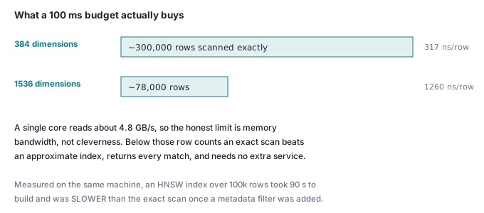
- A 100 ms budget buys roughly 480 MB of vectors: about 300,000 rows at 384 dimensions, or about 78,000 rows at 1536 dimensions.
- 1,000,000 vectors at 1536 dimensions is 8.2 GB in SQLite and took 32.6 seconds per query from Python. At that size the constraint is memory, not cleverness.
- The naive-versus-vectorised gap is a Python problem, not a universal one. In Node, the "naive" loop over ordinary JS arrays was as fast as a packed
Float32Array— 30.9 ms against 30.1 ms at 100,000 rows. - pgvector with no index at all matched a hand-written typed-array loop (about 30 ms at 100,000 × 384) and beat plain SQL over
float4[]by 60x.
How slow is brute force at 100k vectors?
Vectors are stored pre-normalised as float32 BLOBs, one row each, so cosine similarity is a plain dot product. The Python column scans the SQLite table and uses math.sumprod; the Node column scans one contiguous Float32Array.
| Rows | Dim | SQLite size | Bytes/row | Python scan (median) | Node packed (median) |
|---|---|---|---|---|---|
| 1,000 | 384 | 2.1 MB | 2,056 | 5.9 ms | 0.76 ms |
| 10,000 | 384 | 20.5 MB | 2,053 | 56.6 ms | 3.24 ms |
| 100,000 | 384 | 205.3 MB | 2,053 | 728.7 ms | 30.1 ms |
| 1,000,000 | 384 | 2,053 MB | 2,053 | 15,231 ms | 377 ms |
| 1,000 | 1,536 | 8.2 MB | 8,208 | 23.5 ms | 1.30 ms |
| 10,000 | 1,536 | 82.0 MB | 8,202 | 277.1 ms | 11.5 ms |
| 100,000 | 1,536 | 820.2 MB | 8,202 | 3,318.7 ms | 126.5 ms |
| 1,000,000 | 1,536 | 8,202 MB | 8,202 | 32,580 ms | 3,929 ms |
Storage is boringly predictable: 2,053 bytes per row at 384 dimensions against a theoretical 1,536, and 8,202 against 6,144. SQLite's per-row overhead is about 500 bytes and it does not grow. You can budget disk with a multiplication.
Latency is not predictable in the same way, because two different things go wrong at the two ends of the table. At 1,000 rows a query is fast in any language. At 1,000,000 × 1,536 the working set is 8.2 GB on a 16 GB laptop, and the Node figure swung from 2.57 s to 5.98 s across runs — that spread is the memory system, not the CPU.
Why is the Python version seventeen times slower?
This is where the expected story broke. The received advice is "replace the naive loop with a vectorised one and the problem goes away". Measured per dot product, in microseconds:
| Implementation | 384 dim | 1,536 dim |
|---|---|---|
sum(x*y for x, y in zip(a, b)) over lists |
8.48 µs | 37.82 µs |
math.sumprod over lists |
1.63 µs | 7.07 µs |
math.sumprod over tuples |
1.62 µs | 6.95 µs |
math.sumprod over array('f') |
5.23 µs | 20.77 µs |
Two things here are worth more than the headline 5.2x.
numpy was not installed on this machine, and it turned out not to be needed. math.sumprod, added in Python 3.12, is a C-level sum of products in the standard library. It is the whole vectorisation story for anyone who wants one dependency fewer.
Its fast path only covers lists and tuples. Feed it the array('f') you naturally use for compact float32 storage and it is 3.2x slower, because every element gets boxed into a Python float on the way in. Scanning 100,000 vectors took 622.2 ms from array('f') and 215.4 ms from lists — 2.89x faster. That speedup costs 7.3x the memory: 1,688 bytes for an array('f') of 384 floats against 12,344 bytes for the equivalent list once you count the float objects. Compact storage and fast arithmetic are in direct conflict here, and nobody tells you that.
Now the part that contradicts the advice outright. In Node, at 100,000 × 384:
| Implementation | Median | Spread |
|---|---|---|
Packed Float32Array, one contiguous buffer |
30.1 ms | 29.2 – 40.1 ms |
| "Naive" loop over ordinary JS arrays | 30.9 ms | 30.2 – 38.2 ms |
node:sqlite row scan, decode per row |
297.4 ms | 176.3 – 314.3 ms |
The naive version is not slower. V8 stores arrays of numbers as unboxed doubles and compiles the inner loop to the same machine code, so there is no gap to close. The gap people attribute to "vectorisation" is really the gap between an interpreter that boxes every float and one that does not. Choosing the right language erases it; so does math.sumprod. What does still cost you 10x in Node is pulling rows out of SQLite one at a time — the arithmetic was never the problem.
Where exactly does brute force stop working?
Define the threshold: 100 ms median for a single query, which is about the slowest a search box can be before typing feels laggy. Single core, in process, vectors already resident.
| Dim | Rows | Vector bytes | Median | ns/row | Verdict |
|---|---|---|---|---|---|
| 384 | 150,000 | 230 MB | 47.8 ms | 319 | fine |
| 384 | 200,000 | 307 MB | 63.4 ms | 317 | fine |
| 384 | 250,000 | 384 MB | 79.3 ms | 317 | fine |
| 384 | 300,000 | 461 MB | 95.0 ms | 317 | at the limit |
| 1,536 | 25,000 | 154 MB | 31.3 ms | 1,252 | fine |
| 1,536 | 50,000 | 307 MB | 63.1 ms | 1,263 | fine |
| 1,536 | 75,000 | 461 MB | 94.3 ms | 1,257 | at the limit |
| 1,536 | 100,000 | 614 MB | 205.1 ms | 2,051 | over |
The per-row cost is 317 ns at 384 dimensions and 1,260 ns at 1,536 — a ratio of 3.97 against a dimension ratio of 4.00. Cost is linear in bytes scanned, and both work out to 4.8 GB/s on one core. So the rule is: divide 480 MB by your bytes per vector.
One honest caveat, because it nearly fooled us. Earlier passes of this same sweep showed a "cache cliff" at 300 MB where ns/row jumped from 320 to 800. Re-running on a settled machine made it vanish up to 300,000 rows. It was memory pressure left over from previous allocations in the same session, not a property of the hardware. The 1,536-dimension cliff at 614 MB did reproduce in every pass, which is why it is in the table and the other one is not.
And the language matters more than the index. The same sweep in Python ran at 5,509 ns/row — the 100 ms budget crosses at about 18,000 rows, not 300,000.
What does a vector database actually add?
Measured on PostgreSQL 17.11 with pgvector 0.8.6, 100,000 genuinely distinct random 384-dimension vectors, 157 MB heap.
| Query path | Median | Spread | Notes |
|---|---|---|---|
Plain float4[] cosine via unnest, no extension |
1,862 ms | 1,495 – 1,891 ms | pure SQL |
pgvector <=>, sequential scan, no index |
56.7 ms | 47.2 – 84.0 ms | 1 core |
pgvector <=>, sequential scan, 2 parallel workers |
51.8 ms | 44.0 – 63.0 ms | exact |
HNSW index, ef_search = 40 |
4.8 ms | 3.5 – 6.2 ms | approximate |
HNSW index, ef_search = 400 |
21.7 ms | 18.9 – 32.8 ms | approximate |
The first row is the real warning. Writing cosine similarity as SQL over float4[] with unnest is 33x slower than the same brute force through pgvector's SIMD kernel, and 60x slower than an index. If you have decided to avoid a vector database, do not also avoid a vector type.
The index is not free. Building HNSW with m = 16, ef_construction = 64 on those 100,000 rows took 90.6 seconds single-threaded, and the index is 195 MB against a 157 MB table — 1.25x the data it indexes. Every insert pays into that graph too.
Then metadata filtering, which is where this gets interesting. Adding WHERE cat = 3 to select one category of ten:
| Query | Median | Rows returned of 10 |
|---|---|---|
| HNSW, filter applied after the index scan | 8.05 ms | 5 |
HNSW with hnsw.iterative_scan = relaxed_order |
42.80 ms | 10 |
| Exact scan with the same filter | 7.94 ms | 10 |
The default behaviour silently returned half the rows we asked for: the index finds its nearest neighbours, then the filter throws most of them away. pgvector 0.8's iterative_scan fixes the count and costs 5x the latency — at which point it is slower than the exact scan, which was already fast because the ordinary B-tree index on cat cut the candidate set to 10,000 rows. Filtered vector search is the case where ANN indexes are weakest and brute force is strongest, and most real applications filter.
Does any of this tell you the search is good?
No, and here is the proof that random vectors cannot answer that question.
Recall against the exact top-10, measured on the same data:
ef_search |
Median | recall@10 |
|---|---|---|
| 10 | 2.58 ms | 0.018 |
| 40 | 4.76 ms | 0.064 |
| 100 | 9.70 ms | 0.145 |
| 400 | 21.73 ms | 0.345 |
Six percent recall at the default setting would be a catastrophic result if it meant anything. It does not. A control run of the identical harness with the index disabled returned recall 1.000, so the measurement is sound — the data is the problem. On uniformly random vectors in 384 dimensions, distances concentrate: the nearest neighbour sits at cosine distance 0.7458 while the mean is 1.0002 with a standard deviation of 0.0510, and the first thousand neighbours span just 0.095 of distance between them. There is no cluster structure for a navigable graph to exploit, because random noise has none.
Real embeddings do have that structure, which is the entire reason HNSW works in practice. Take every latency and size number in this article; ignore every recall number. That is the honest boundary of a benchmark with no embedding model behind it.
So when do you actually need one?
Below roughly 300,000 vectors at 384 dimensions, or 78,000 at 1,536, a scan in a compiled-or-JIT language is under 100 ms and exact. You get no recall cliff, no index build, no extra 195 MB, no tuning parameter, and filtering makes it faster rather than breaking it. Store the vectors as float32 BLOBs next to your data — the same argument as full-text search that works on a plane, where the index living inside SQLite is the point.
You need the real thing when: your vectors no longer fit in memory on one machine (the wall we hit at 8.2 GB); you are past a few million rows and cannot throw cores at it; you need concurrent queries per second rather than one at a time, where a 50 ms scan per query caps you at 20 QPS per core; or you need sharding and replication over the vectors themselves. Those are infrastructure problems, and they arrive later than the marketing suggests.
Before adding one, check the cheaper lever: fewer, better chunks beat a faster index over bad ones, which is chunking a document without destroying its meaning. Halving your chunk count halves your scan time exactly as reliably as any index, and it improves the results instead of approximating them.
Check it yourself
No network, no API key, no model call, no numpy. Needs Python 3.12+ for math.sumprod. Save as vecdemo.py:
import array, heapq, math, random, sqlite3, statistics, sys, time

DIM, TOPK, RUNS = 384, 10, 7
BUDGET_MS = 100.0

def unit(dim, rnd):
    v = array.array("f", (rnd.gauss(0, 1) for _ in range(dim)))
    n = math.sqrt(math.sumprod(v, v))
    for i in range(dim):
        v[i] /= n
    return v

def search(rows, q):                      # rows: list of array('f')
    best = []
    for i, a in enumerate(rows):
        s = math.sumprod(a, q)            # C-level dot product, no numpy
        if len(best) < TOPK:
            heapq.heappush(best, (s, i))
        elif s > best[0][0]:
            heapq.heapreplace(best, (s, i))
    return best

def search_naive(rows, q):
    best = []
    for i, a in enumerate(rows):
        s = sum(x * y for x, y in zip(a, q))
        if len(best) < TOPK:
            heapq.heappush(best, (s, i))
        elif s > best[0][0]:
            heapq.heapreplace(best, (s, i))
    return best

print(f"python {sys.version.split()[0]}  sqlite {sqlite3.sqlite_version}  dim {DIM}")
print("RANDOM vectors -- speed only, says nothing about retrieval quality\n")

rnd = random.Random(7)
pool = [unit(DIM, rnd).tobytes() for _ in range(4096)]

print(f"{'rows':>8} {'db MB':>7} {'B/row':>6} {'sqlite scan':>12} "
      f"{'in-RAM':>9} {'naive':>10} {'ns/row':>7}")
for n in (1_000, 10_000, 50_000, 100_000, 200_000, 300_000):
    db = sqlite3.connect(":memory:")
    db.execute("CREATE TABLE vecs(id INTEGER PRIMARY KEY, v BLOB NOT NULL)")
    db.executemany("INSERT INTO vecs VALUES (?,?)",
                   ((i, pool[i % 4096]) for i in range(n)))
    size = (db.execute("PRAGMA page_count").fetchone()[0]
            * db.execute("PRAGMA page_size").fetchone()[0])

    rows = []
    for (blob,) in db.execute("SELECT v FROM vecs"):
        a = array.array("f"); a.frombytes(blob); rows.append(a)

    qr = random.Random(99)
    def timed(fn, arg, runs):
        out = []
        for _ in range(runs):
            q = unit(DIM, qr)
            t = time.perf_counter()
            fn(arg, q)
            out.append((time.perf_counter() - t) * 1000)
        return statistics.median(out)

    def scan_db(db, q):
        best = []
        for (i, blob) in db.execute("SELECT id, v FROM vecs"):
            a = array.array("f"); a.frombytes(blob)
            s = math.sumprod(a, q)
            if len(best) < TOPK: heapq.heappush(best, (s, i))
            elif s > best[0][0]: heapq.heapreplace(best, (s, i))
        return best

    t_db = timed(scan_db, db, RUNS)
    t_ram = timed(search, rows, RUNS)
    t_naive = timed(search_naive, rows, 3) if n <= 100_000 else float("nan")
    flag = "  <- over budget" if t_ram > BUDGET_MS else ""
    print(f"{n:>8} {size/1e6:>7.1f} {size/n:>6.0f} {t_db:>10.1f}ms "
          f"{t_ram:>7.1f}ms {t_naive:>8.1f}ms {t_ram*1e6/n:>7.0f}{flag}")
    db.close()

print(f"\nBudget {BUDGET_MS:.0f} ms. Divide it by the ns/row above to get the row")
print("count where brute force stops being interactive on YOUR machine.")
python3 vecdemo.py
On the M3 laptop above that prints:
python 3.14.6  sqlite 3.53.4  dim 384
RANDOM vectors -- speed only, says nothing about retrieval quality

    rows   db MB  B/row  sqlite scan    in-RAM      naive  ns/row
    1000     2.1   2056        5.9ms     5.4ms     13.3ms    5353
   10000    20.5   2053       61.9ms    55.1ms    128.5ms    5509
   50000   102.7   2053      309.0ms   280.7ms    657.8ms    5615  <- over budget
  100000   205.3   2053      626.7ms   563.4ms   1321.2ms    5634  <- over budget
  200000   410.6   2053     1285.9ms  1190.9ms      nanms    5954  <- over budget
  300000   615.9   2053     2011.2ms  1826.1ms      nanms    6087  <- over budget
That is the Python wall at about 18,000 rows, and it is the number most people actually measure before concluding they need a vector database. Then do the experiment that matters. Change rows.append(a) to rows.append(a.tolist()), and give search a list-form query by adding q = list(q) as its first line so that both sides of math.sumprod are lists. The same scan gets about 2.8x faster (2.89x and 2.82x on two separate runs here), at 7.3x the memory, without adding a single dependency — which is the whole article in one edit.